PythonモジュールPandasで時間信号の実効値を計算する方法についてソースコード付きでまとめました。
## 【はじめに】実効値とは
実効値とは、時間信号の平均的な大きさ(強さ)を表す値です。
つまり、時間変動する信号が平均的にどの程度の影響を与えているかを評価できます。
周期信号の場合
時間信号 が周期信号の場合、周期
 のときの実効値は以下の式で計算できます。
(1) 
非周期信号の場合
時間信号が非周期信号の場合、周期のときの実効値は以下の式で計算できます。
(2) 
実効値は「時間信号の二乗平均の平方根(rms : root mean square)」を計算しているため、rms値とも呼ばれます。
| – | 関連記事 |
|---|---|
| 1 | 【信号処理】実効値の計算式・計算例(Excel、Pythonなど) |
## 【Pandas】時間信号データの実効値を計算
時間信号データ(CSV)を読み込んで、実効値を計算してみます。
ついでに平均値、最大値も計算してグラフにプロットしてみます。
| – | 読み込んだデータ |
|---|---|
| CSV | current.csv |
current.csv
time,current
-6,0
-5.8,1
-5.6,0
-5.4,0
︙
0,0
0.2,1
0.4,2
︙
2.4,13
2.6,12
2.8,16
︙
サンプルコード
# -*- coding: utf-8 -*-
import os
import pandas as pd
import matplotlib
import matplotlib.pyplot as plt
import numpy as np
import math
from scipy.optimize import curve_fit
import ntpath
# 読み込むCSVファイルのパス
csv_path = "C:/prog/python/auto/current.csv"
save_path = "C:/prog/python/"
# 空のデータフレームを作成
df = pd.DataFrame({})
# CSVファイルのロードし、データフレームへ格納
df = pd.read_csv(csv_path, encoding="UTF-8", skiprows=0)
# 電流値の列データを取り出し
Its = df.loc[:, "current"]
# 経過時間の列データを取り出し
times = df.loc[:, "time"]
N = Its.size # サンプル数
Irms = np.sqrt(np.square(Its).mean()) # 実効値の計算
# 電流の最大値、平均値を計算
Imax = Its.max()
Imean = Its.mean()
# 計算結果の表示
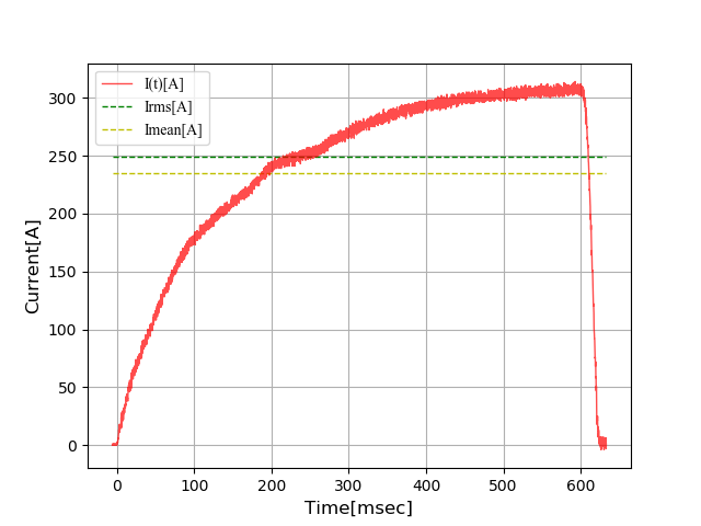
print("Irms[A]=", Irms) # Irms[A] = 249.061976770524
print("Imax[A]=", Imax) # Imax[A] = 314
print("Imean[A]=", Imean) # Imean[A] = 235.10106382978722
# 保存先パスが存在しなければ作成
if not os.path.exists(save_path):
os.mkdir(save_path)
# グラフ化
ax = plt.axes()
plt.rcParams['font.family'] = 'Times New Roman' # 全体のフォント
plt.rcParams['axes.linewidth'] = 1.0 # 軸の太さ
# 電流値をプロット
plt.plot(times, Its, lw=1, c="r", alpha=0.7, ms=2, label="I(t)[A]")
# 電流の実効値を水平線でプロット
plt.hlines(Irms, min(times), max(times), ls='--', color="g", lw=1, label="Irms[A]")
plt.hlines(Imean, min(times), max(times), ls='--',
color="y", lw=1, label="Imean[A]")
# グラフの保存
plt.legend(loc="best") # 凡例の表示(2:位置は第二象限)
plt.xlabel('Time[msec]', fontsize=12) # x軸ラベル
plt.ylabel('Current[A]', fontsize=12) # y軸ラベル
plt.grid() # グリッドの表示
plt.legend(loc="best") # 凡例の表示
plt.savefig(save_path + "current.png")
plt.clf()
| – | 関連記事 |
|---|---|
| 1 | 【Pandas入門】データ分析のサンプル集 |
| 2 | 【Python入門】サンプル集・使い方 |

コメント